Create Semantic Differential (SD) Plots

sdRplot is an R function (in the sdRgraph R package) that can be used for creating Semantic Differential (SD) inventory plots.

Usage

sdRplot(nx, sl, ny, x)

Arguments

nx

The number of levels in each of the the SD scales in the inventory, e.g., 5

sl

The scale labels given as a list, e.g. c("SA","A","N","A","SA")

ny

The number of descriptor items in the inventory

x

The data matrix with the first column (col1) containing the low-end descriptors of the SD scales, the second column (col2) containing the high-end descriptors of the SD scales, and the third column and beyond (col3-onwards) containing the mean scale values for each group. The names of the columns (col 3 and above) of the data matrix (e.g., dimnames(x)[[2]][3:ncol(x)])) are used for labelling the groups in the legend.

Value

The SD plot of the data summarized in matrix x.

Examples

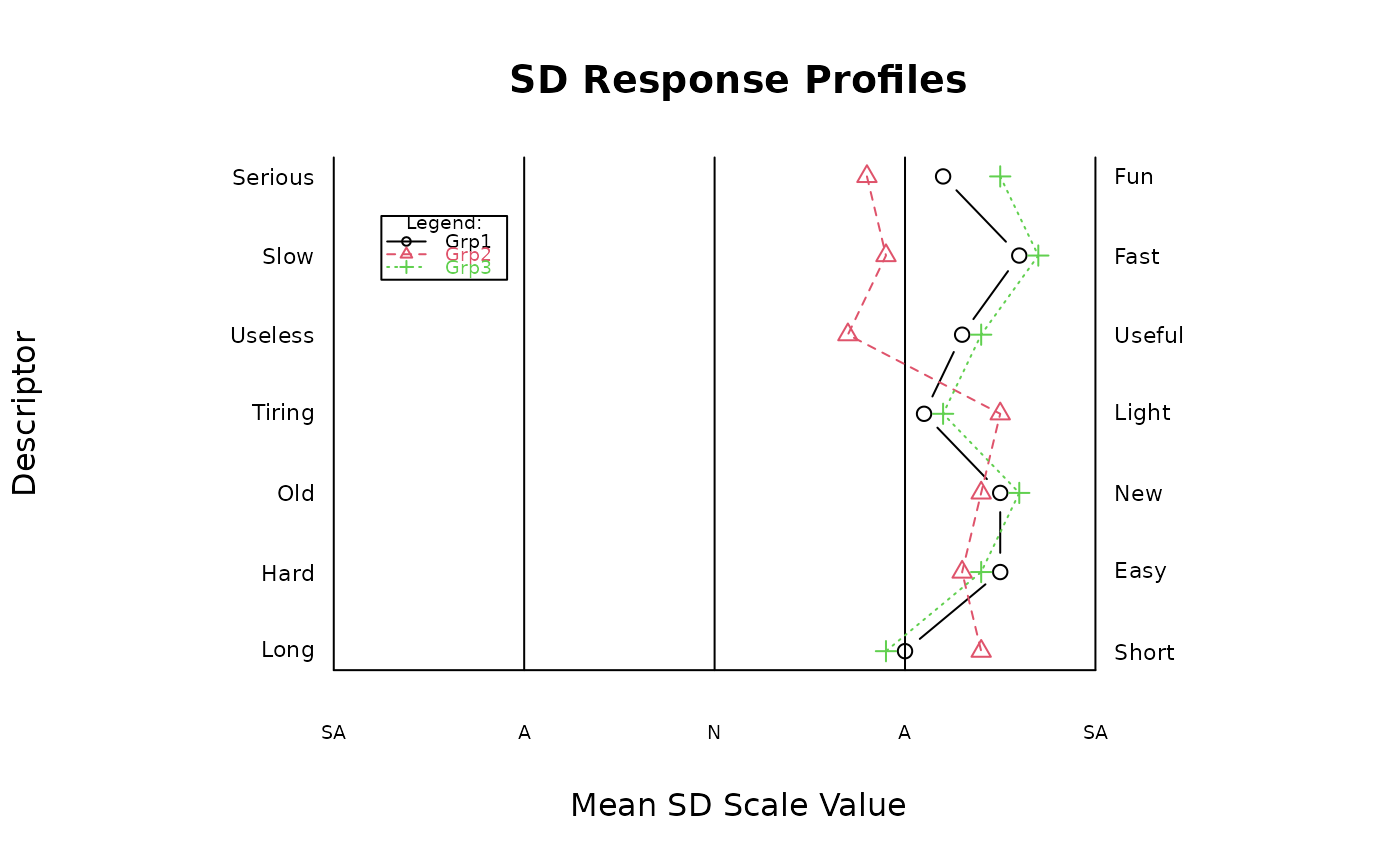
low<-c("Serious","Slow","Useless","Tiring","Old","Hard","Long")
high<-c("Fun","Fast","Useful","Light","New","Easy","Short")
scale<-c("SA","A","N","A","SA")
grp1means<-c(4.2,4.6,4.3,4.1,4.5,4.5,4.0)
grp2means<-c(3.8,3.9,3.7,4.5,4.4,4.3,4.4)
grp3means<-c(4.5,4.7,4.4,4.2,4.6,4.4,3.9)
data<-matrix(
 cbind(low,high,grp1means,grp2means,grp3means),
 nrow=7,ncol=5,byrow=FALSE,
 dimnames=list(c("I1","I2","I3","I4","I5","I6","I7"),
               c("Low","High","Grp1","Grp2","Grp3"))
)
sdRplot(5,scale,7,data)